Plotting dlfs
daisy-02-plotting-dlfs.RmdThere is a general plot function plot_dlf that handles
both single files and list of files as returned by
read_dlf.
Plotting data from a directory of dlf files
To get started we will read some dlf files with
read_dlf
data_dir <- system.file("extdata", package="daisyrVis")
dlfs <- read_dlf(file.path(data_dir, "annual"))
names(dlfs)
#> [1] "Annual-FN/HourlyP-Annual-FN-2-2b"
#> [2] "Annual-FN/HourlyP-Annual-FN-2-3b"
#> [3] "Annual-FN/HourlyP-Annual-FN-2-4b"
#> [4] "Annual-FN/HourlyP-Annual-FN-2-5b"
#> [5] "Annual-Tracer/HourlyP-Annual-Tracer-2-2b"
#> [6] "Annual-Tracer/HourlyP-Annual-Tracer-2-3b"
#> [7] "Annual-Tracer/HourlyP-Annual-Tracer-2-4b"
#> [8] "Annual-Tracer/HourlyP-Annual-Tracer-2-5b"
plot_dlf can only plot multiple dlf files with the same
columns. The data we just read contains data from two different log
types and multiple scenarios
colnames(dlfs[[1]]@data)
#>  [1] "year"                   "month"                  "mday"
#>  [4] "hour"                   "Min_Surface_Fertilizer" "Min_Soil_Fertilizer"
#>  [7] "Deposition"             "Matrix_Leaching"        "Biopore_Leaching"
#> [10] "Soil_Drain"             "Biopore_Drain"          "Surface_Loss"
#> [13] "Min_Surface"            "Min_Soil"               "Min_Biopores"
#> [16] "Error"                  "Mineralization"         "Immobilization"
#> [19] "Crop_Uptake"            "Volatilization"         "N2O_Nitrification"
#> [22] "Denitrification"        "Fixated"                "Org_Fertilizer"
#> [25] "Seed"                   "Harvest"                "Residuals_Surface"
#> [28] "Residuals_Soil"         "Org_Surface"            "Org_Soil"
#> [31] "Crop"                   "time"
colnames(dlfs[[8]]@data)
#>  [1] "year"              "month"             "mday"
#>  [4] "hour"              "Spray"             "Deposit"
#>  [7] "Harvest"           "Dissipate"         "Litter Decompose"
#> [10] "Litter Transform"  "Surface Decompose" "Surface Transform"
#> [13] "Runoff"            "Leak matrix"       "Leak biopores"
#> [16] "Biopore drain"     "Soil drain"        "Surface drain"
#> [19] "External"          "Uptake"            "Soil Decompose"
#> [22] "Soil Transform"    "Snow"              "Canopy"
#> [25] "Litter"            "Surface"           "Soil"
#> [28] "Biopores"          "Error"             "time"
So we need to select a subset of the files that have the same columns.
dlfs <- dlfs[c(1, 2, 3, 4)]
names(dlfs)
#> [1] "Annual-FN/HourlyP-Annual-FN-2-2b" "Annual-FN/HourlyP-Annual-FN-2-3b"
#> [3] "Annual-FN/HourlyP-Annual-FN-2-4b" "Annual-FN/HourlyP-Annual-FN-2-5b"
dlfs <- drop_dir_from_names(dlfs)
dlfs <- strip_common_prefix_from_names(dlfs)
names(dlfs)
#> [1] "2b" "3b" "4b" "5b"
These dlfs contain annually logged variables related to field nitrogen
colnames(dlfs[[1]]@data)
#>  [1] "year"                   "month"                  "mday"
#>  [4] "hour"                   "Min_Surface_Fertilizer" "Min_Soil_Fertilizer"
#>  [7] "Deposition"             "Matrix_Leaching"        "Biopore_Leaching"
#> [10] "Soil_Drain"             "Biopore_Drain"          "Surface_Loss"
#> [13] "Min_Surface"            "Min_Soil"               "Min_Biopores"
#> [16] "Error"                  "Mineralization"         "Immobilization"
#> [19] "Crop_Uptake"            "Volatilization"         "N2O_Nitrification"
#> [22] "Denitrification"        "Fixated"                "Org_Fertilizer"
#> [25] "Seed"                   "Harvest"                "Residuals_Surface"
#> [28] "Residuals_Soil"         "Org_Surface"            "Org_Soil"
#> [31] "Crop"                   "time"
We can plot all the variables, or a subset. Here we plot “Surface_Loss” and “Denitrification”.
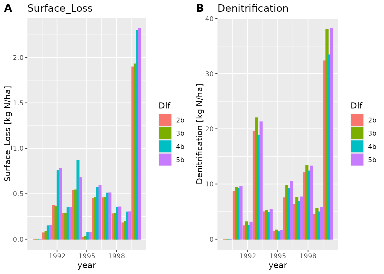 Notice how
 plot_dlf plots each variable in a separate sub
plot, and each scenario (AKA dlf) with a different color.
We can also make a line or points plot, or combine the plots types
plot_dlf(dlfs, "year", y_vars, "lines")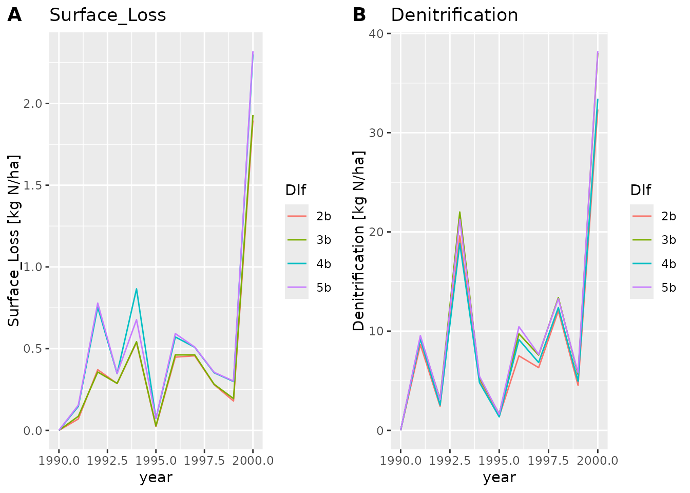
plot_dlf(dlfs, "year", y_vars, "points")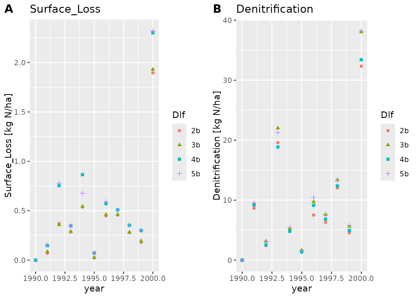
plot_dlf(dlfs, "year", y_vars, "lines-points-bar")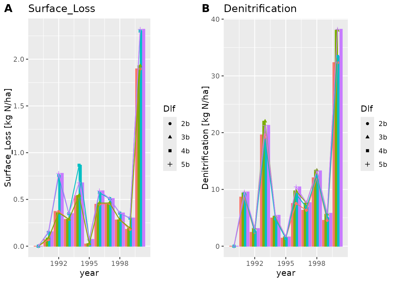
The lines and points plot types are usually better suited when we
have more data points. To see this we will load another dlf file using
read_dlf
path <- file.path(data_dir, "hourly/P2D-Daily-Soil_Chemical_110cm.dlf")
dlf <- read_dlf(path)
colnames(dlf@data)
#>  [1] "year"                    "month"
#>  [3] "mday"                    "hour"
#>  [5] "In_Matrix"               "In_Biopores"
#>  [7] "Leak_Matrix"             "Leak_Biopores"
#>  [9] "Biopores to matrix"      "Matrix to biopores"
#> [11] "Tillage"                 "Drain_Soil"
#> [13] "Drain_Biopores"          "Drain_Biopores_Indirect"
#> [15] "External"                "Uptake"
#> [17] "Decompose"               "Transform"
#> [19] "Content"                 "Biopores"
#> [21] "Error"                   "time"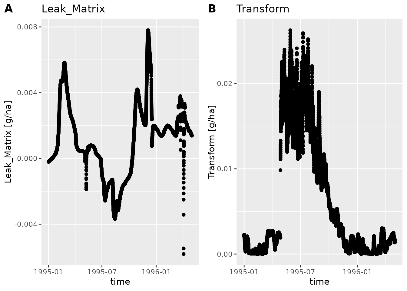
If we only want to plot a part of the time period we can use
subset_dlf
summer95 <- subset_dlf(dlf, "1995-06-01", "1995-08-31")
plot_dlf(summer95, "time", y_vars, "lines", title_suffix=" - Summer of '95")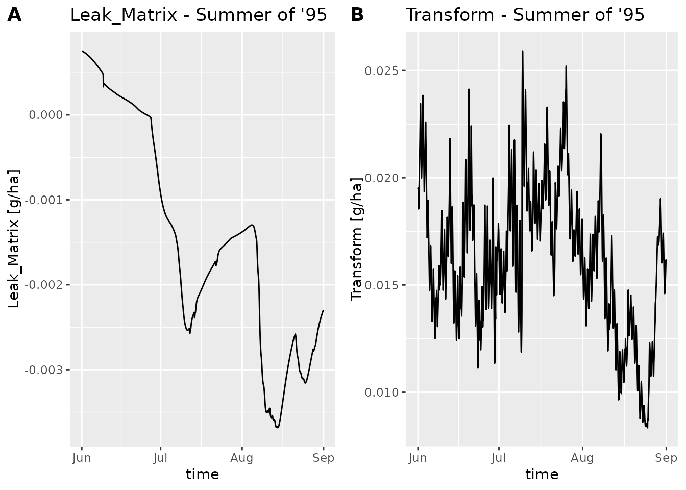
Plotting Daisy spawn output
To get started we will read some dlf files with
read_dlf
data_dir <- system.file("extdata", package="daisyrVis")
path <- file.path(data_dir, "daisy-spawn-like")
dlfs <- read_dlf(path)
names(dlfs)
#> [1] "FWater200-Y" "Harvest"
As before we need to ensure that we only plot dlfs with the same
columns. In this case read_dlf has done most of the work
for us and we can directly index the list of dlfs
colnames(dlfs$Harvest@data)
#>  [1] "year"    "month"   "day"     "column"  "crop"    "stem_DM" "dead_DM"
#>  [8] "leaf_DM" "sorg_DM" "stem_N"  "dead_N"  "leaf_N"  "sorg_N"  "WStress"
#> [15] "NStress" "WP_ET"   "HI"      "sim"     "time"
plot_dlf(dlfs$Harvest, "time", "leaf_DM", "lines")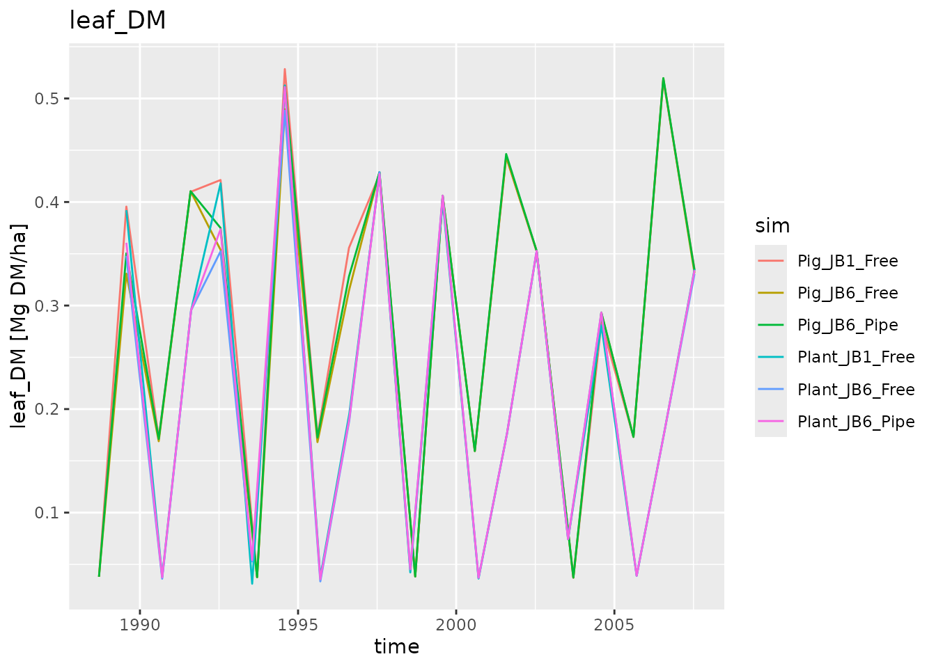
We can of course also plot the other log type
colnames(dlfs$`FWater200-Y`@data)
#>  [1] "year"                         "month"
#>  [3] "mday"                         "hour"
#>  [5] "Precipitation"                "Irrigation"
#>  [7] "Potential evapotranspiration" "Actual evapotranspiration"
#>  [9] "Matrix percolation"           "Biopore percolation"
#> [11] "Matrix drain flow"            "Biopore drain flow"
#> [13] "Runoff"                       "Biopore water"
#> [15] "Soil matrix water"            "Surface water"
#> [17] "sim"                          "time"
plot_dlf(dlfs$`FWater200-Y`, "time", "Irrigation", "bar")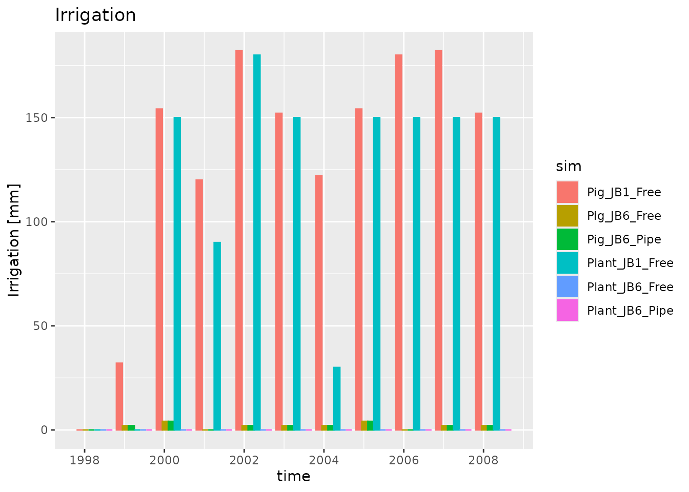
Plotting depth distributed output
To get started we will read a dlf file with read_dlf
data_dir <- system.file("extdata", package="daisyrVis")
path <- file.path(data_dir, "daily/DailyP/DailyP-Daily-WaterFlux.dlf")
dlf <- read_dlf(path)
head(dlf)
#>   year month mday hour       time z        q
#> 1 1990     4    2    0 1990-04-02 0 0.686972
plot_dlf does not yet support plotting depth data.
Instead you have to use plot_dlf_depth
plot_dlf_depth(dlf, "q")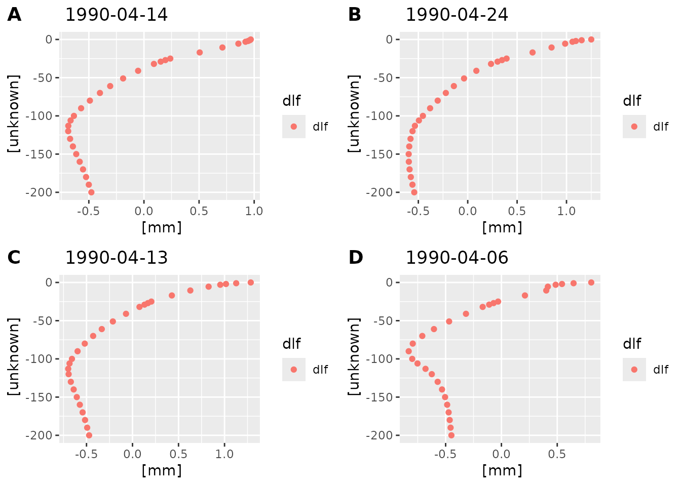 By default
 plot_dlf_depth selects four time points at
random. You can also pass the desired time points
plot_dlf_depth(dlf, "q", c("1990-04-23", "1990-04-27"))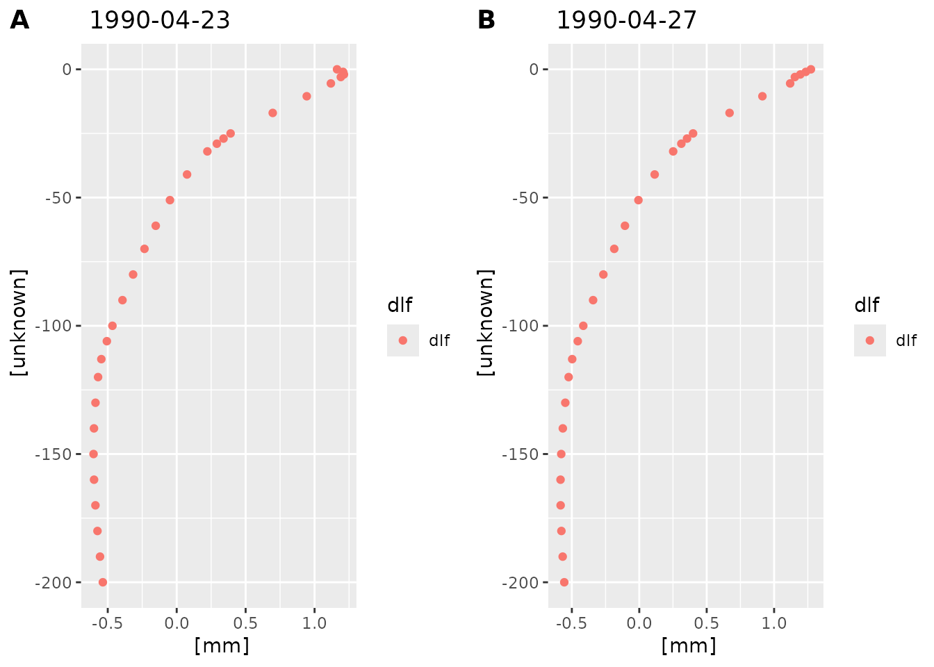
Depth distributed data is often better visualized by animating it.
This can be done with animate_dlf. Try running
example(animate_dlf).